Introduction to ddfr

This vignette provides a short introduction to the ddfr package. I apologize for it not being typeset beautifully, however as I created this package for an exercise sheet submission at university, I’m bound by time constraints.

Nevertheless, this vignette, together with the documentation usable within R by ? should be more than enough in order to get started with this package. Every function listed below has a dedicated help page in R which should hopefully provide you with all relevant information. You can also check out the Reference on the website.

Lastly, thanks a lot for checking out my package! :)

Overview

After having installed the package (most probably from GitHub), it can be loaded in R using the following command:

library(ddfr)

The focus of the package is working with the custom S4 class ddf which provides a convenient way to work with discrete distributions with finite support in R.

It has three slots called supp, probs and desc which, in that order, give the support of the distribution, the corresponding probabilities and a short description of the respective distribution. They can all be accessed using the getters supp(), probs() and desc(). For the description there is also a setter such that it can easily be changed:

mydist <- ddf(1:6, rep(1 / 6, 6), "A first description")
mydist
#> A first description 
#> 
#> Support:
#> [1] 1 2 3 4 5 6
#> 
#> Probabilities:
#> [1] 0.1666667 0.1666667 0.1666667 0.1666667 0.1666667 0.1666667
supp(mydist)
#> [1] 1 2 3 4 5 6
desc(mydist) <- "This description fits better"
mydist
#> This description fits better 
#> 
#> Support:
#> [1] 1 2 3 4 5 6
#> 
#> Probabilities:
#> [1] 0.1666667 0.1666667 0.1666667 0.1666667 0.1666667 0.1666667

Creating new `ddf` objects

Manually

The intended way to create custom new ddf objects is to use the provided function with the same name. It takes as its arguments a numerical vector specifying the support of the distribution, a second numerical vector of the same length containing the corresponding probabilities and lastly, an optional description of the distribution.

For example, to create a distribution modeling a single throw of a fair six-sided dice, one can use:

ddf(1:6, rep(1 / 6, 6), "A distribution modeling a single dice throw")
#> A distribution modeling a single dice throw 
#> 
#> Support:
#> [1] 1 2 3 4 5 6
#> 
#> Probabilities:
#> [1] 0.1666667 0.1666667 0.1666667 0.1666667 0.1666667 0.1666667

Note that the probabilities have to approximately sum up to \(1\) or otherwise the function throws an error. While this might change in the future, in the current implementation, the error has to be less than 1e-10:

# Probabilities don't sum up to ≈1
try(ddf(1, 1 - 1e-10))
#> Error in validObject(.Object) : 
#>   invalid class "ddf" object: probabilities have to sum up to approximately 1

# This works
ddf(1, 1 - 1e-11)
#> A discrete distribution with finite support 
#> 
#> Support:
#> [1] 1
#> 
#> Probabilities:
#> [1] 1

In case one does not have probabilities, but absolute frequencies instead, one can also use ddf_from_frequencies() as an alternative. For example, the following creates a ddf object from hypothetical counts of throwing a six-sided dice one hundred times:

ddf_from_frequencies(1:6, c(19, 14, 17, 18, 15, 17), "My dice throws")
#> My dice throws 
#> 
#> Support:
#> [1] 1 2 3 4 5 6
#> 
#> Probabilities:
#> [1] 0.19 0.14 0.17 0.18 0.15 0.17

As one can see, the arguments are mostly the same except for passing the frequencies instead of the probabilities as the second argument.

For more details on both methods please consult the documentation of ddf() and ddf_from_frequencies(), respectively.

Using the already implemented distributions

ddfr already provides you with a large amount of common discrete distributions. The below list shows the currently implemented discrete distributions with finite support. To learn more about any single one of them, use the help in R, e.g. ?bin(). Once again I’d like to mention the Reference as it might also be a convenient way to find a specific distribution you’re looking for.

Discrete uniform distribution as unif()
Bernoulli distribution as bernoulli()
Binomial distribution as bin()
Rademacher distribution as rademacher()
Benford’s law as benford()
Zipf distribution as zipf()
Hypergeometric distribution as hypergeometric()
Negative hypergeometric distribution as negative_hypergeometric()
Beta-binomial distribution as beta_binomial()

Furthermore, there are also functions to create approximations of the following three discrete distributions with countably infinite support.

Poisson distribution as pois()
Negative binomial distribution as negative_bin()
Geometric distribution as geometric()

The approximation works by finding a large enough number \(r > 0\) such that cutting of the support after \(r\) yields an overall probability which is within a given range \(\epsilon\) of \(1\). The default value for \(\epsilon\) is 1e-10, however this can be customized using the eps argument. Unless the normalize argument is manually set to FALSE (by default it is TRUE) the approximation is then also normalized such that the sum of all probabilities becomes precisely one. The following examples demonstrate this, however, for further details you might also want to check out the respective documentation of the function you’re using.

# Approximation of the Poisson distribution
# to demonstrate the `normalize` argument
p <- pois(20, normalize = FALSE)

# Not equal to one (but still pretty close):
1 - sum(probs(p))
#> [1] 9.051593e-11

# Note how the `normalize` argument here could be omitted
# since it is `TRUE` by default
p_normalized <- pois(20, normalize = TRUE)

# Now the summed probabilities are equal to one:
1 - sum(probs(p_normalized))
#> [1] 0


# For most cases, something like this should suffice
geometric(0.8)
#> (Approximation of a) geometric distribution with p = 0.8, starting at 0 
#> 
#> Support:
#>  [1]  0  1  2  3  4  5  6  7  8  9 10 11 12 13 14
#> 
#> Probabilities:
#>  [1] 8.00000e-01 1.60000e-01 3.20000e-02 6.40000e-03 1.28000e-03 2.56000e-04
#>  [7] 5.12000e-05 1.02400e-05 2.04800e-06 4.09600e-07 8.19200e-08 1.63840e-08
#> [13] 3.27680e-09 6.55360e-10 1.31072e-10

# However, you can of course increase the accuracy if you want to
geometric(0.8, eps = .Machine$double.eps)
#> (Approximation of a) geometric distribution with p = 0.8, starting at 0 
#> 
#> Support:
#>  [1]  0  1  2  3  4  5  6  7  8  9 10 11 12 13 14 15 16 17 18 19 20 21
#> 
#> Probabilities:
#>  [1] 8.000000e-01 1.600000e-01 3.200000e-02 6.400000e-03 1.280000e-03
#>  [6] 2.560000e-04 5.120000e-05 1.024000e-05 2.048000e-06 4.096000e-07
#> [11] 8.192000e-08 1.638400e-08 3.276800e-09 6.553600e-10 1.310720e-10
#> [16] 2.621440e-11 5.242880e-12 1.048576e-12 2.097152e-13 4.194304e-14
#> [21] 8.388608e-15 1.677722e-15

From other `ddf` objects

Lastly, there is also the possibility to use already existing ddf objects to create new ones. Currently there are only two functions for doing so.

The first one is the generic method - with which the support of a distribution can be multiplied with \(-1\):

-bin(5, 0.8)
#> Binomial distribution with parameters n = 5 and p = 0.8, multiplied with -1 
#> 
#> Support:
#> [1] -5 -4 -3 -2 -1  0
#> 
#> Probabilities:
#> [1] 0.32768 0.40960 0.20480 0.05120 0.00640 0.00032

The second one is the function shift() with which the support of a distribution can be shifted by a specified amount:

shift(unif(3), 3)
#> Discrete uniform distribution on {1, ..., 3}, shifted by 3 
#> 
#> Support:
#> [1] 4 5 6
#> 
#> Probabilities:
#> [1] 0.3333333 0.3333333 0.3333333

Analysis of distributions

ddfr provides many ways to analyze a given distribution. This section only lists the corresponding functions. For details, the respective documentations should hopefully suffice.

Central tendency

Expected value as expected_value() or generic mean()
Medians as medians() (plural form as they aren’t necessarily unique)
Modes as modes() (plural form as they aren’t necessarily unique)

Dispersion

Standard deviation as standard_deviation()
Variance as variance()
Interquartile range as iqr()
Range as distribution_range()

Moments

\(n\)-th raw moment as moment()
\(n\)-th central moment as central_moment()
\(n\)-th standardized moment as standardized_moment()

Besides this, there are also additional functions for calculating some specific often used moments (besides the already previously mentioned variance):

Skewness as skew()
Kurtosis as kurtosis()
Excess kurtosis as excess_kurtosis()

Quantiles

Quantiles as quantiles()
Percentiles as percentile()
Deciles as decile()
Quartiles as quartile()

Entropy

Entropy as entropy()

Report

In case one wants to quickly get an overview of the considered distribution, there is also the function report() which, as the name suggests, writes a report on the given distribution involving most of the above properties. The following example demonstrates this (please not that for the purpose of better readability, the output is printed as normal text):

cat(report(bin(15, 0.7)))

The given distribution could be described as “Binomial distribution with parameters n = 15 and p = 0.7”.

It has a mean/expected value of 10.5, the average of its mode(s) is given by 11 and the average of its median(s) is 11. It is a unimodal distribution.

Regarding its dispersion, calculating its variance yields 3.15 which implies a standard deviation of 1.77482393492988. When talking about other measures of variability, one can assert that the distribution’s range constitutes 15 over its 16 elements, whereas its interquartile range is given by 3 since the (smallest) first quartile is 9 and the (largest) third quartile is 12.

It has a skewness of -0.225374467927603 (measured using Fisher’s moment coefficient of skewness) and with an excess kurtosis of -0.0825396825396827 (and hence kurtosis of 2.91746031746032) it is a platykurtic, also called platykurtotic, distribution.

Lastly, it can be noted that its entropy, measured in bits, is 2.86637454085645.

Creating new objects from `ddf` distributions

Creating `R` functions

One can use pmf and cdf to get R functions behaving like the probability mass function and cumulative distribution function for a given distribution, respectively. Especially the first of these two is rather useful as it can be used to get the probability of any number:

# Probability of 5 in a binomial distribution with parameters n = 10 and p = 0.7
pmf(bin(10, 0.7))(5)
#> [1] 0.1029193

Note that this also works for numbers which are not part of a distribution’s support, in which case the function simply returns \(0\):

pmf(bin(10, 0.7))(3.5)
#> [1] 0

Sampling

Use samples() to create samples based on a distribution. For example, one can simulate 10 fair dice throws as follows:

samples(unif(6), 10)
#>  [1] 2 1 5 2 2 4 4 3 6 6

This function was also used to generate the frequency table for dice throws above in the “Creating new ddf objects” section.

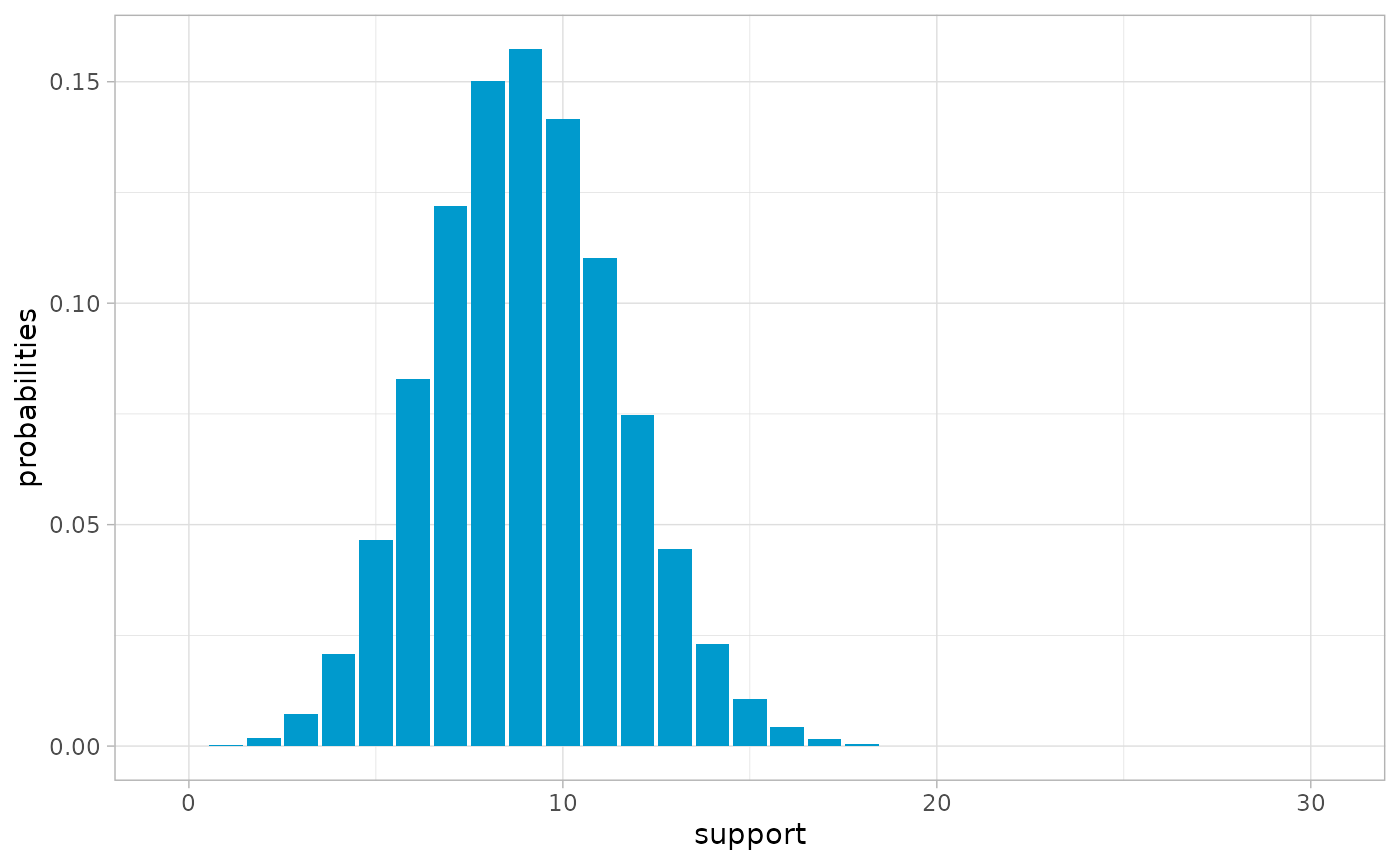
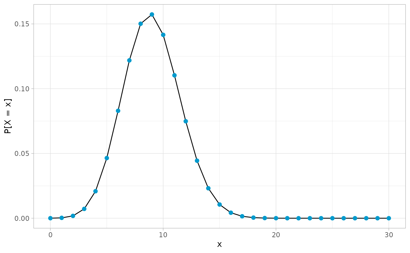
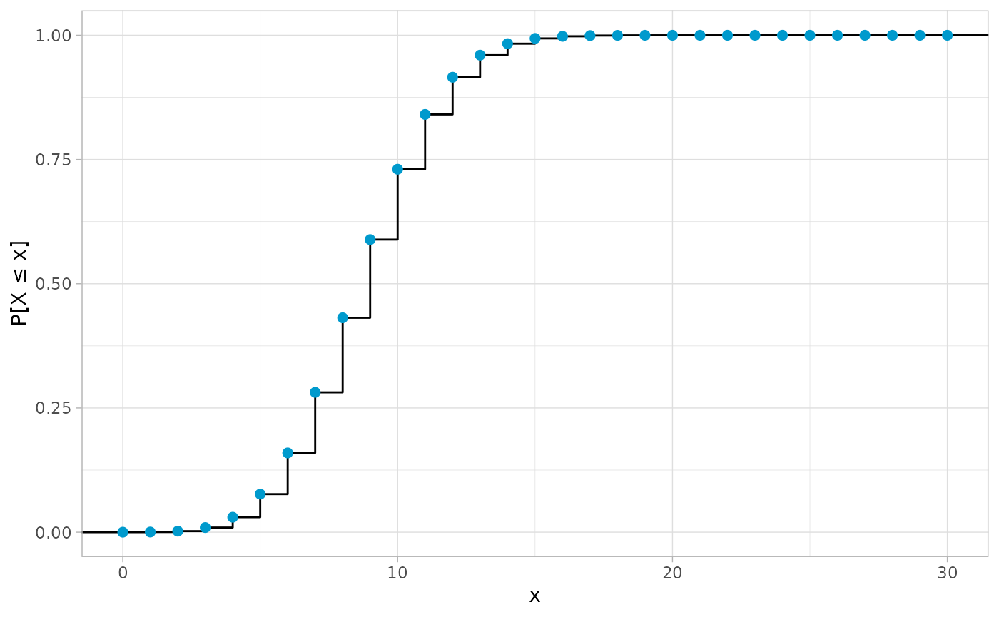
Plotting

ddfr also provides extensive plotting capabilities via the three functions plot(), plot_pmf() and plot_cdf(). The first one of these is once again a generic for the S4 class ddf.

At least when it comes to plots, an image is worth a thousand words, so here are all three functions in action:

plot(bin(30, 0.3))

plot_pmf(bin(30, 0.3))

plot_cdf(bin(30, 0.3))

Convolutions

Lastly, there is the possibility to calculate convolutions of distributions. For example, to compute the distribution of the sum of two six-sided dice when tossed together, one can use

conv(unif(6), unif(6))
#> A convolution 
#> 
#> Support:
#>  [1]  2  3  4  5  6  7  8  9 10 11 12
#> 
#> Probabilities:
#>  [1] 0.02777778 0.05555556 0.08333333 0.11111111 0.13888889 0.16666667
#>  [7] 0.13888889 0.11111111 0.08333333 0.05555556 0.02777778

# Short hand using *
unif(6) * unif(6)
#> A convolution 
#> 
#> Support:
#>  [1]  2  3  4  5  6  7  8  9 10 11 12
#> 
#> Probabilities:
#>  [1] 0.02777778 0.05555556 0.08333333 0.11111111 0.13888889 0.16666667
#>  [7] 0.13888889 0.11111111 0.08333333 0.05555556 0.02777778

The second example shows how the generic * has also been defined for objects from the ddf class to quickly convolve distributions.

The function conv_n() calculates the \(n\)-fold convolution of a distribution with itself, see ?conv_n() for details.

Lastly, there is also the function convolve_cpp() which is the underlying implementation for the convolution using Rcpp for better performance. It is not really intended for use with ddfr objects directly, but might still be useful in other applications.